Data Vault 2.0 emerged from years of production implementations, codifying the patterns that consistently delivered results.
Dan Linstedt released the original Data Vault specification in 2000. The hub-link-satellite modeling approach solved a real problem: how do you integrate multiple source systems without creating brittle star schemas that collapse as soon as a source system changes its primary key structure for the first time? The modeling framework was solid. But Linstedt left implementation details open to interpretation, and teams filled the gaps differently.
By 2013, enough organizations had built Data Vaults that clear patterns emerged. Some teams generated surrogate keys using sequences. Others used MD5 hashes. Some loaded data nightly in batches. Others streamed changes continuously. Performance varied wildly based on these choices, and nobody could agree on which approach was “correct” Data Vault.
Data Vault 2.0 standardized what the original specification left undefined. The hub-link-satellite modeling stayed identical. But now you have explicit rules for hash key generation, standardized loading procedures, and architectural patterns.
This article breaks down what changed between versions, why those changes matter for real implementations, and where Data Vault 2.0 still leaves you making difficult trade-offs.
The Three Pillars: Modeling, Architecture, and Methodology
Data Vault 2.0 organizes its specification around three pillars: Modeling, Architecture, and Methodology. The original version was only based around modeling and left you to figure out the rest.
Modeling Pillar: Same Structures, Better Definitions
The modeling pillar defines how you represent data. Hubs store business keys for entities. Links capture relationships between business entities. Satellites hold descriptive attributes and their change history.
Data Vault 1.0 defined these structures but didn’t specify how to handle edge cases. Version 2.0 added formal definitions for:
Multi-active satellites handle cases where a single business key has multiple concurrent values for the same attribute. A person with two active phone numbers requires a multi-active satellite because it is not possible to represent “phone number” as a single value at a single point in time.
Link satellites store attributes that describe relationships rather than entities. When did this customer-product relationship start? Who created it? These attributes describe the relationship itself, so they go in a link satellite attached to the customer-product link.
Point-in-time (PIT) tables pre-materialize temporal joins across multiple satellites. Building these got mentioned in Data Vault 1.0 discussions, but the 2.0 specification includes explicit guidance on grain, update frequency, and when PIT tables actually improve performance versus just consuming storage.
Bridge tables flatten complex link structures for common query patterns. If your reporting layer constantly joins through five links to answer a single question, a bridge table can pre-compute those joins.
Architecture Pillar: Platform-Specific Implementation
The architecture pillar addresses the fact that Data Vault implementations run on platforms with wildly different characteristics.
Data Vault 1.0 assumed relational databases with strong ACID guarantees. By 2013, teams were implementing Data Vault on Hadoop, loading from message queues, and running workloads on NoSQL stores.
Data Vault 2.0 includes patterns for distributed computing frameworks where you can’t rely on database transactions, cloud data warehouses with platform-specific optimization features, and stream processing where data arrives continuously instead of in daily batch loads.
Platform-specific implementation guides translate these patterns into concrete configurations. A Snowflake implementation tells you exactly how to structure clustering keys for hash-based lookups. A Databricks implementation maps the same logical Data Vault structures to Delta tables with different physical optimization strategies.
This matters because discovering these optimizations through production failures wastes months. Implementation guides tell you upfront how to avoid expensive automatic reclustering or suboptimal partition strategies.
Methodology Pillar: Agile Delivery Practices
The methodology pillar defines how teams organize work when building Data Vault implementations. This entire pillar was new in version 2.0.
Data Vault modeling is inherently incremental. You can build one hub in week one, add satellites in week two, and connect through links in week three. Each component integrates with existing structures without requiring rework.
Data Vault 2.0 includes sprint planning templates that break data warehouse development into two-week increments, user story patterns for data warehouse features, testing approaches for data warehouse components, and deployment practices for promoting changes through environments.
Technical Improvements That Actually Matter
Several technical patterns in Data Vault 2.0 addressed problems that plagued 1.0 implementations.
Hash Keys Replace Composite Natural Keys
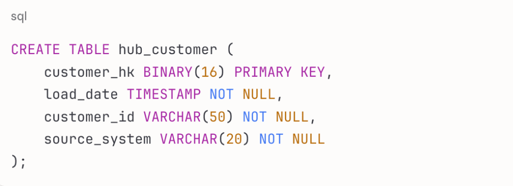
Every hub in Data Vault 2.0 uses a hash key generated from the business key. If your customer business key is a composite of customer_id and source_system, you hash those values together using MD5 or SHA-256 to create a fixed-length hash key.
Here’s what a customer hub looks like:
CREATE TABLE hub_customer (
customer_hk BINARY(16) PRIMARY KEY,
load_date TIMESTAMP NOT NULL,
customer_id VARCHAR(50) NOT NULL,
source_system VARCHAR(20) NOT NULL
);
Join performance improves because you’re joining on fixed-length 16-byte or 32-byte values instead of variable-length composite keys. Parallel loading becomes simpler because multiple processes can independently generate identical hash values without coordinating. Sensitive data gets obscured without separate masking procedures.
But hashing creates debugging challenges. When you find a data discrepancy, you can’t look at the hash key and know what customer it represents. Many implementations include business keys in at least one satellite for each hub, even though it’s technically redundant, just to make debugging possible.
Persistent Staging Areas Capture Raw Extracts
Data Vault 2.0 formalizes persistent staging areas that keep every raw data extract without truncation.
Most traditional ETL processes extract data from sources, load it to a staging table, transform it, write results to a warehouse, then truncate the staging table. If you need to troubleshoot a data issue later, the raw extract is gone.
Persistent staging keeps everything. Staging tables become a permanent archive of every extract, including malformed records, duplicates, and data that failed validation rules. When you discover a revenue discrepancy from three months ago, persistent staging lets you query the exact extract from that date.
The downside is storage cost. Most teams implement retention policies—keep staging data for 90 or 180 days, then archive to cheaper storage or delete it.
Point-in-Time Tables Pre-Compute Temporal Joins
PIT tables materialize temporal joins during the load process instead of at query time.
A customer might have satellites for contact information, credit rating, and purchase preferences. To answer “what did this customer look like on March 15, 2024?” you need to join all three satellites with temporal logic. Do this for every customer in every query, and performance suffers.
A PIT table performs these joins during the nightly load and stores the results. Your query becomes a simple key-value lookup. PIT tables can improve query performance substantially—temporal queries that previously took 45 seconds can drop to under 2 seconds.
But you need to choose grain carefully. Daily PIT snapshots for every customer create massive tables. Most teams don’t need PIT tables initially. Build your Data Vault without them. When specific query patterns show clear performance problems, add PIT tables for those patterns.
Business Vault Layers Separate Raw from Derived Data
The business vault concept separates raw source data from calculated fields and business rules.
The raw vault loads data exactly as received from sources. No transformations, no business rules, no derived calculations. The business vault applies standardization, calculations, and enrichments that don’t exist in any source system.
This separation keeps the raw vault auditable. When someone questions where a number came from, you can point to the exact source record. When business rules change, you modify the business vault without touching raw vault structures.
The challenge is that this doubles your table count. Most teams start with just a raw vault and add business vault views incrementally.
Why Teams Pick Data Vault 2.0 Over Dimensional Modeling
Data Vault works better than dimensional modeling for specific scenarios.
Multiple Source Integration Without Redesign
Adding a new source system to a star schema often requires redesigning fact and dimension tables. In Data Vault, you create new satellites for the new source. Each source gets its own set of satellites, preserving source-specific context. The hub stays the same—it just identifies customers.
Consider a healthcare company that merges with a competitor. They need to integrate two completely different ERP systems. Their dimensional model requires months of redesign work and breaks dozens of downstream reports. A Data Vault implementation adds the new source through new satellites without touching existing structures.
Full Audit Trails for Regulatory Requirements
Dimensional models handle history through slowly changing dimension (SCD) patterns. Type 2 SCDs keep history by adding effective_date and end_date columns. This works until you have hundreds of dimension attributes that change independently.
Data Vault satellites automatically track every attribute change with load timestamps. You don’t design for audit trails—they’re built into the structure. Reconstructing historical state means filtering satellite rows to records effective at a specific timestamp.
Platform Migration Without Logical Redesign
Data Vault’s platform-agnostic modeling means your logical design stays consistent across different database platforms. The same hub-link-satellite structures that work on SQL Server work on Snowflake. Physical optimization changes—clustering strategies, partition schemes, indexing approaches—but the logical model doesn’t.
Dimensional designs often embed platform-specific assumptions. A star schema designed for SQL Server columnstore indexes might need restructuring for Snowflake’s micro-partitions. Data Vault’s simpler table structures adapt to new platforms more cleanly.
Where Data Vault 2.0 Still Leaves You Making Hard Choices
Data Vault 2.0 standardized many implementation details, but some decisions remain platform-specific and context-dependent.
Satellite granularity: You could put all customer attributes in one large satellite, or split them by change frequency. More granular satellites reduce row size but increase query complexity. The specification doesn’t prescribe this—teams choose based on change patterns and query patterns.
PIT table timing: The specification tells you how to build PIT tables but not when they’re worth the overhead. Most teams build PIT tables reactively—wait for query performance complaints, identify common temporal join patterns, add targeted PIT tables.
History retention: Satellites accumulate unlimited history by default. A customer who’s been updating their profile monthly for ten years has 120 rows in various satellites. Data Vault 2.0 includes patterns for archiving old satellite versions, but deciding how much history to keep online depends on query patterns and compliance requirements.
Cut Data Vault Development Time with Automation
Building Data Vault structures manually means writing repetitive loading procedures for every hub, link, and satellite. Each hub needs deduplication logic based on hash keys. Each satellite requires change detection that compares incoming records against the latest version.
For a mid-sized implementation with 50 hubs and 200 satellites, you’re writing hundreds of similar-but-not-identical loading procedures. Change a business key definition, and you’re updating hash key generation logic across dozens of tables.
Metadata-driven automation platforms generate loading code, orchestration workflows, and documentation automatically. Define your hubs, links, and satellites once in metadata. When source systems change or business rules evolve, update the metadata and regenerate. Your implementation stays aligned with requirements without manual code maintenance across hundreds of procedures.
These platforms work across Snowflake, Microsoft Fabric, Databricks, and traditional databases. Platform-specific optimizations get applied automatically—Snowflake deployments use clustering keys and streams, Fabric deployments use Delta tables and notebooks.
Teams using automated development deliver working Data Vault implementations in weeks instead of quarters because they’re not building from scratch. Developers focus on business logic and data quality rules instead of writing boilerplate loading procedures.
Speed Up Your Data Vault Implementation
Building Data Vault 2.0 architectures manually takes months of repetitive development work. Teams spend time writing loading procedures, managing change detection logic, and maintaining documentation across dozens or hundreds of tables.
WhereScape automates this entire process through metadata-driven development. Define your hubs, links, and satellites once, and our platform generates the loading code, orchestration workflows, and documentation automatically. When source systems change or business rules evolve, you update the metadata and regenerate — your implementation stays aligned with requirements without manual code maintenance.
The automation works across platforms. Whether you’re building on Snowflake, Microsoft Fabric, Databricks, or traditional databases, WhereScape applies Data Vault 2.0 patterns optimized for each platform’s specific capabilities.
Request a demo to see how WhereScape eliminates the manual work in Data Vault implementations. Get working data warehouses in weeks rather than months.
FAQ
Data Vault 2.0 standardized implementation details that the original specification left undefined. The core modeling approach with hubs, links, and satellites remained identical between versions. Version 2.0 added explicit rules for hash key generation using MD5 or SHA-256, formalized persistent staging areas that preserve raw extracts, introduced point-in-time tables for pre-computed temporal joins, and created the business vault layer for separating raw from derived data. The specification also added two entirely new pillars beyond modeling: architecture patterns for different database platforms and agile methodology practices for organizing development work. Teams using Data Vault 1.0 had to figure out these implementation details through trial and error, while 2.0 provides proven patterns upfront.
Hash keys in Data Vault 2.0 convert variable-length composite business keys into fixed-length binary values of 16 bytes for MD5 or 32 bytes for SHA-256. Join performance improves substantially because databases optimize fixed-length key operations far better than joins on composite keys with multiple varchar columns. Parallel loading becomes simpler because multiple processes can independently generate identical hash values from the same business key without coordinating through a central sequence generator. Hash keys also provide automatic data masking for sensitive business keys without separate obfuscation procedures. The trade-off is debugging difficulty, as you cannot look at a hash value and immediately identify which business entity it represents, which is why most implementations include business keys in at least one satellite despite the technical redundancy.
Point-in-time tables should be added reactively after identifying specific query performance problems rather than built upfront for every entity. Most teams start their Data Vault implementation without PIT tables and monitor query patterns during production use. When temporal queries consistently take 30-45 seconds to join multiple satellites across thousands of customers, that specific pattern justifies a PIT table that pre-computes those joins during nightly loads and reduces query time to under 2 seconds. Building PIT tables for every possible temporal join pattern wastes storage and maintenance effort on tables that may never get queried. The grain of PIT tables also matters substantially, as daily snapshots for every customer across years of history create massive tables that might exceed the performance benefit they provide.
Data Vault handles multiple source systems through source-specific satellites attached to the same hub, allowing each source to contribute attributes without redesigning existing structures. When a healthcare company merges with a competitor running completely different ERP systems, a dimensional model requires months of fact and dimension table redesign that breaks downstream reports. A Data Vault implementation simply adds new satellites for the new source while keeping all existing hubs, links, and satellites unchanged. Each source maintains its own context and change history in separate satellites, eliminating the need to reconcile conflicting attribute definitions or forcing one source’s structure onto another. This architecture also preserves full audit trails showing exactly which source system provided each attribute value at each point in time, which regulatory requirements often demand.
Persistent staging areas preserve every raw data extract permanently instead of truncating staging tables after successful loads. Traditional ETL processes extract data from sources, load it to staging, transform it, write to the warehouse, then truncate staging tables to prepare for the next load. When data discrepancies appear three months later, the original extract is gone and teams cannot verify what the source system actually sent. Persistent staging keeps complete archives of every extract including malformed records, duplicates, and data that failed validation rules, enabling teams to query the exact state of source data from any historical date. The primary trade-off is storage cost, which most teams manage through retention policies that keep staging data for 90 to 180 days before archiving to cheaper storage or deletion.